Overview
This is the optimization half of a two-part study. The screening stage is Which Variables Matter?
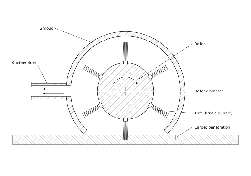
Using an efficient screening method, a consumer product company was able to use data to confidently reduce seven variables down to three for a household vacuum brush roller assembly they were designing. Those screening results told the team what to pay attention to, but not what to set those variables to — and said nothing at all about what each setting would cost to build. This case study is an example of how efficient experimentation can optimize both at once.
With only three factors remaining, a 2³ factorial with five replicates was the right design for the team. It let them answer both questions simultaneously: what is the best-performing roller at the lowest cost? It also freed them to set the variables that don't affect cleaning performance — brush speed and carpet penetration — for noise, motor wear or aesthetics instead. Without factorial experimentation, none of that would have been possible.
By optimizing cost against performance simultaneously, the team found that two design changes cost the same eight cents per roller assembly — but one of them buys 3.7 times more cleaning performance than the other.
Without this experiment they would likely have chosen the inferior design without ever realizing it — and spent the same money for a quarter of the benefit.
The Challenge
Knowing which variables matter is the start of a design problem, not the end of one. A typical screening experiment reveals two critical pieces of information: which variables matter, and which direction to go. In this case it pointed toward more tufts per roller and thinner individual tufts, with core diameter worth a look. However, it does not tell you how many tufts. And it certainly does not tell you whether the last few points of performance are worth what they cost to manufacture.
That second question is the one that actually decides a product. Every variable on the shortlist has a price attached to it — more material, more machine time, a bigger mold — and the cheapest way to make a vacuum clean better is rarely the most obvious way. An engineering team optimizing on performance alone will happily specify a brush roller that rarely survives a downstream cost assessment.
So the follow-up experiment had to optimize two responses at once: pickup, the percentage of test soil lifted from the carpet, and cost per unit, what the brush roller costs to make. Optimizing either one alone is straightforward arithmetic. Optimizing both together is the real job, and it is the part a designed experiment does that intuition cannot.
The Experimental Approach
Three variables survived screening, and each earned its place for a different reason:
- Number of tufts — the largest single driver of pickup in the screening study, at 51% of the variation.
- Tuft diameter — the second largest at 42%, and thinner turned out to be better.
- Core diameter — barely moves pickup at 3%, but it drives the cost of the most expensive part in the assembly, which is why it was carried forward into the cost optimization.
With the field of variables narrowed this far, the best design for optimizing both cost and performance is a complete 2³ factorial — only eight configurations. The benefit of running the screening design is now paying off: with only three factors to carry forward, a full factorial delivers the most important advantage of factorial experimentation — revealing interactions between factors if they exist, and producing a robust model for predicting performance.
Each configuration was run five times, for 40 runs. The same logic as the screening stage applied: runs are cheap, and replication buys the precision to separate real differences from noise. Here it bought something specific as well — enough pure error to test whether the interactions were real, which is the assumption the entire optimization would rest on.
Side note: the cost per unit is simulated data built from published resin and monofilament pricing, injection-molding conversion costs and staple-set tufting rates, applied to each configuration's geometry. It is a defensible order-of-magnitude estimate layered onto measured performance data to make the trade-off visible. Treat the pickup numbers as findings and the cost numbers as a reasonable model of what those findings would cost to build.
Inputs · variables tested
Core Diameter
25 mm → 34 mm
Tuft Diameter
2 mm → 4 mm
No. of Tufts
66 → 86
Process
Carpet pickup
Outputs · what we measured
Response
Pickup [%]
Response
Cost per Unit [$]
The Design
Forty runs — eight configurations, each repeated five times — measuring pickup as a percentage of test soil removed, with a modeled cost per unit attached to each configuration's geometry.
| Run | Std | Core Diameter(mm) | Tuft Diameter(mm) | No. of Tufts | Pickup[%] | Cost per Unit[$] |
|---|---|---|---|---|---|---|
| 1 | 5 | 25 mm | 2 mm | 86 | 72.5 | 1.0276 |
| 2 | 7 | 25 mm | 4 mm | 86 | 53 | 1.0362 |
| 3 | 5 | 25 mm | 2 mm | 86 | 72.7 | 1.0276 |
| 4 | 5 | 25 mm | 2 mm | 86 | 68.7 | 1.0276 |
| 5 | 6 | 34 mm | 2 mm | 86 | 79.1 | 1.1086 |
| 6 | 7 | 25 mm | 4 mm | 86 | 50.5 | 1.0362 |
| 7 | 3 | 25 mm | 4 mm | 66 | 26.3 | 0.9522 |
| 8 | 8 | 34 mm | 4 mm | 86 | 55.5 | 1.1172 |
| 9 | 2 | 34 mm | 2 mm | 66 | 56.1 | 1.0266 |
| 10 | 2 | 34 mm | 2 mm | 66 | 52.5 | 1.0266 |
| 11 | 5 | 25 mm | 2 mm | 86 | 72.4 | 1.0276 |
| 12 | 7 | 25 mm | 4 mm | 86 | 53.4 | 1.0362 |
| 13 | 6 | 34 mm | 2 mm | 86 | 78.2 | 1.1086 |
| 14 | 2 | 34 mm | 2 mm | 66 | 53.7 | 1.0266 |
| 15 | 6 | 34 mm | 2 mm | 86 | 76.2 | 1.1086 |
| 16 | 4 | 34 mm | 4 mm | 66 | 37.2 | 1.0332 |
| 17 | 6 | 34 mm | 2 mm | 86 | 78 | 1.1086 |
| 18 | 4 | 34 mm | 4 mm | 66 | 36.4 | 1.0332 |
| 19 | 8 | 34 mm | 4 mm | 86 | 57.6 | 1.1172 |
| 20 | 6 | 34 mm | 2 mm | 86 | 76.3 | 1.1086 |
| 21 | 7 | 25 mm | 4 mm | 86 | 48.9 | 1.0362 |
| 22 | 1 | 25 mm | 2 mm | 66 | 49 | 0.9456 |
| 23 | 1 | 25 mm | 2 mm | 66 | 49.6 | 0.9456 |
| 24 | 8 | 34 mm | 4 mm | 86 | 56.1 | 1.1172 |
| 25 | 3 | 25 mm | 4 mm | 66 | 30.1 | 0.9522 |
| 26 | 5 | 25 mm | 2 mm | 86 | 72.2 | 1.0276 |
| 27 | 8 | 34 mm | 4 mm | 86 | 59.8 | 1.1172 |
| 28 | 2 | 34 mm | 2 mm | 66 | 54.6 | 1.0266 |
| 29 | 4 | 34 mm | 4 mm | 66 | 33.4 | 1.0332 |
| 30 | 1 | 25 mm | 2 mm | 66 | 47.6 | 0.9456 |
| 31 | 4 | 34 mm | 4 mm | 66 | 36.8 | 1.0332 |
| 32 | 1 | 25 mm | 2 mm | 66 | 48.8 | 0.9456 |
| 33 | 3 | 25 mm | 4 mm | 66 | 28.2 | 0.9522 |
| 34 | 1 | 25 mm | 2 mm | 66 | 47.6 | 0.9456 |
| 35 | 3 | 25 mm | 4 mm | 66 | 30.4 | 0.9522 |
| 36 | 7 | 25 mm | 4 mm | 86 | 53.4 | 1.0362 |
| 37 | 3 | 25 mm | 4 mm | 66 | 28 | 0.9522 |
| 38 | 2 | 34 mm | 2 mm | 66 | 55.2 | 1.0266 |
| 39 | 8 | 34 mm | 4 mm | 86 | 58.4 | 1.1172 |
| 40 | 4 | 34 mm | 4 mm | 66 | 35.2 | 1.0332 |
40 runs · Randomized run order · Execute in run order to guard against drift
Results & Insights
Bottom line
No. of Tufts, Tuft Diameter, and Core Diameter drive 100% of the impact you measured on Pickup. Focus improvement effort here first.
Pareto Diagram
Amber bars = significant (above crimson threshold at α = 0.05). Gray bars can't be told apart from run-to-run noise.
Main Effects
Average response at each factor setting. Steeper slope = stronger lever. Gray lines are within noise.
Analysis of the Variance (ANOVA)
| Factor | Source | Sum of squares | df | Mean square | F | p-value | % of impact | Real effect? |
|---|---|---|---|---|---|---|---|---|
| C | No. of Tufts | 5203 | 1 | 5203 | 2254 | < 0.001 | 55% | Yes |
| B | Tuft Diameter | 3849 | 1 | 3849 | 1668 | < 0.001 | 41% | Yes |
| A | Core Diameter | 378.2 | 1 | 378.2 | 163.9 | < 0.001 | 4.0% | Yes |
| A×C | Core Diam × No. of | 1.60 | 1 | 1.60 | — | — | 0.0% | Can't tell from noise |
| A×B×C | Core Diam × Tuft Diam × No. of | 1.44 | 1 | 1.44 | — | — | 0.0% | Can't tell from noise |
| A×B | Core Diam × Tuft Diam | 0.729 | 1 | 0.729 | — | — | 0.0% | Can't tell from noise |
| B×C | Tuft Diam × No. of | 1.23 | 1 | 1.23 | — | — | 0.0% | Can't tell from noise |
| Error (noise) | 83.09 | 36 | 2.31 | |||||
| Total | 9514 | 39 | ||||||
α = 0.05 · average response = 53.24 · 40 runs
The model accounts for 99.13% of the variation in pickup, and the three variables rank cleanly: number of tufts at 55.1%, tuft diameter at 40.8%, core diameter at 4.0%.
The first thing worth reporting is something that did not happen. None of the interactions were significant. The largest of them moves pickup by 0.40 points, against 22.81 for the biggest main effect — a factor of fifty-seven. The three variables act independently, which is why the two lines below stay parallel instead of converging or crossing.
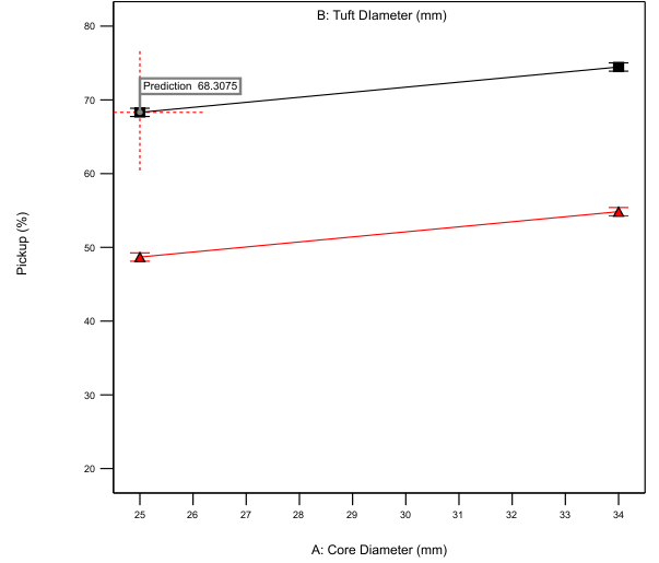
Because interactions can be definitively ruled out — something only a factorial design can establish — the effects simply add. One short equation then predicts the performance of any combination of settings, including combinations that were never explicitly tested. This is a powerful realization: every variable in the model can be tuned to meet some other design goal without the risk of disturbing the others. Remember that the screening stage had to leave interactions unresolved; this full factorial settles them definitively. That builds real confidence for a team that would otherwise be guessing at how their choices affect the rest of the design.
The whole system reduces to one line:
where A is core diameter in millimeters, B is tuft diameter in millimeters and C is the number of tufts — the same letters the design table and the analysis use.
Set it to the combination the team eventually chose — a 25 mm core, 2 mm tufts and 83 tufts — and it returns 68.3% pickup, matching both the optimizer and the hardware. A design that was never built can now be priced and judged before anyone cuts a tool.
With a performance model in hand, the team can now layer the cost side and optimize both. Core diameter drives cost harder than anything else on the list, because a bigger core is more nylon in the molded part:
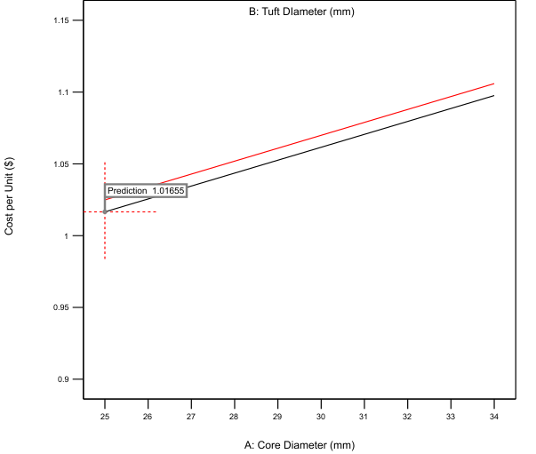
Putting performance and cost side by side is what lets a team balance cost, quality and performance deliberately. Here is what the math said:
- 66 → 86 tufts — gains 22.8 points of pickup for 8.3 cents. $0.0036 per point.
- 4 → 2 mm tuft diameter — gains 19.6 points and saves 0.8 cents. Free — it pays you.
- 25 → 34 mm core — gains 6.2 points for 8.1 cents. $0.0132 per point.
Tuft count and core diameter cost within two-tenths of a cent of each other. Tuft count returns 3.7 times more pickup per dollar. A team working from intuition would very likely have specified the larger core — it is the most visible change, and it does genuinely improve cleaning — and paid the same money for a quarter of the benefit. That is the kind of bad decision a factorial experiment quietly saves you from, and it is either invisible or far too slow to find without one.
Better still is the middle row. Going thinner on the tufts adds nearly twenty points of pickup and costs slightly less, because a thinner tuft is less filament. Performance and cost point the same direction, which almost never happens — and without the experiment it would have been easy to assume the opposite and design the cheaper, worse product on purpose.
Optimizing cost against performance reveals the best available combination. Maximizing pickup alone gives a 34 mm core, 2 mm tufts and 86 tufts — about 77.5% pickup at $1.109. Optimizing pickup and cost together gives a 25 mm core, 2 mm tufts and roughly 83 tufts: 68.3% pickup at $1.017. The last nine points of cleaning performance cost an extra nine cents a unit. This is where structured experiments shine: the team now has efficiently derived metrics that let decision-makers weigh the trade-off in quantitative terms. Review meetings are focused on problems and their solutions, not on intuition or poorly derived models. This is real data, built on real hardware, optimized against real costs.
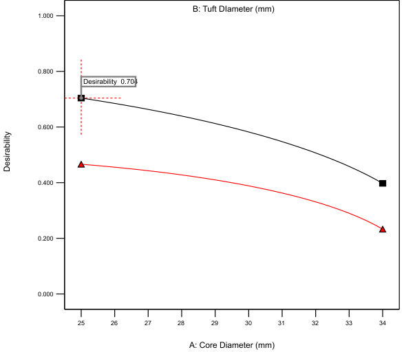
Nobody on this team had to choose between a vacuum that cleans well and one they could afford to build. They found out what each point of performance actually costs — and then they stopped guessing.
Twenty distinct configurations across both stages took a seven-variable design space, found what drives it, resolved how the survivors combine, and produced a costed recommendation a product team could act on. That is the return on treating experimentation as a sequence rather than a single event.
Key Takeaways
- Optimize the objective you actually have — maximizing pickup alone specifies a brush roller that costs nine cents more for performance that might not be necessary for your target market.
- Cost per point of performance is the number that decides — tuft count and core diameter cost the same to change, and one returns 3.7 times more. No amount of engineering judgment produces that ratio without the data.
- Check for interactions before trusting an additive answer — the largest here was fifty-seven times smaller than the largest main effect, which is what makes one short predictive equation legitimate.
- Some changes pay twice — thinner tufts added nearly twenty points of pickup and cost slightly less, a direction intuition tends to get backwards.
- Replication is what answers the objection "is this just noise?" — five repeats per configuration gave the error estimate every interaction test is measured against.
- Screen first, then optimize — twelve configurations found the variables, eight priced them, and neither study would have been enough on its own.
Source. Allen, P. (2020). Design of Experiments for 21st Century Engineers. Lulu.com. ISBN 978-0-244-58450-4, p. 62–71. The Blueprint recreation, the analysis framing and the plain-English reading of the results are original WIS work.